

Written by: Keith Fraga
Edited by: Sydney Wyatt
The California shelter-in-place order due to COVID-19 has been in effect for over a month, with an uncertain end-date. Understanding how the disease is spreading by making predictions based on current data can help health officials in their decision on when to lift the order. There are a number of ways one can analyze the data on COVID-19 cases to model where the epidemic is heading.
Often, statistics on COVID-19 growth rate are given in terms of cumulative cases from the start of the epidemic. As an example using data from the Johns Hopkins COVID-19 resource site, the growth rate in the number of cases in the U.S. quickly surpassed Spain, which has the second highest growth rate, and it is still increasing. How this growth rate changes and ultimately decreases will be a major determining factor for the ending of shelter-in-place orders. Yet, it is difficult to model or uncover the trends in COVID-19 progression through a timeline of total infections, like in Figure 1, due to the exponential nature of the growth of total cases.
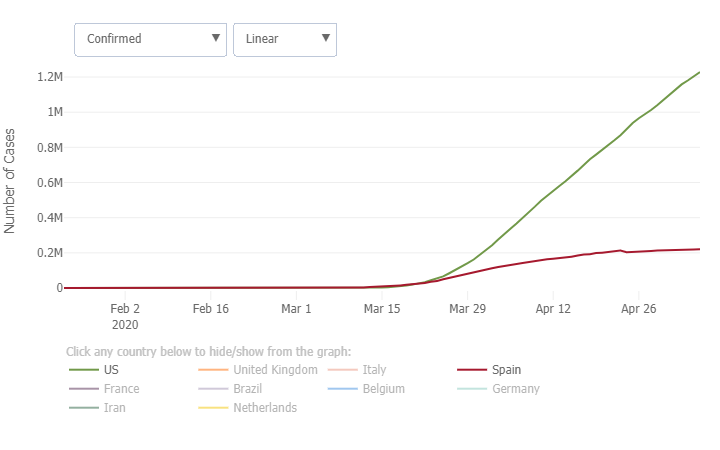
Figure 1: Total number of COVID-19 cases in U.S. (green) and Spain (red) based on data from Johns Hopkins.
In epidemiology, the spread of a disease undergoes an early period of exponential growth. Once the disease progresses to a point where no new infections can occur, the growth rate slows and the cumulative number of cases plateaus. This is called logistic growth, and an example of logistic growth is shown from the 2014-2016 Ebola outbreak data below. Looking at the steepest part in the curve in Figure 2, could we have known that the Ebola outbreak would plateau when it did?
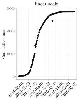
Figure 2: Timeline for the cumulative growth of cases in the 2014-2016 Ebola outbreak.
When there is only data from the middle of the logistic growth curve, it is challenging to predict when the curve will plateau. It is possible to make estimates of when an outbreak could plateau, but this requires looking at the data in a different way, described more below. The ability to predict and model this time to plateau, thereby estimating when the epidemic might be under control, will be a major factor in deciding when normal operations can resume.
‘The virus makes the timeline’
Dr. Anthony Fauci, the NIH infectious disease expert at the center of the U.S. response to COVID-19, gave some insight into interpretation of the outbreak. In a CNN interview on March 25th, Dr. Fauci explained that it is very difficult to know when we can return to normalcy. Further, our attempt to put a deadline on the virus is folly: “You don’t make the timeline, the virus makes the timeline.” How can we understand the virus’ timeline? This question exposes that time may not be the appropriate independent variable to track the epidemic’s progress.
The growth of the virus depends on many factors, but fundamentally it depends on the number of currently infected patients that can transmit the virus. Mathematically, this is captured by modelling the infection growth rate as proportional to the number of currently infected. As more infected cases occur, the faster the outbreak spreads. Time – in days, weeks, or months – since the outbreak is an indirect way to track the virus’s progression. As more time elapses there are more transmission events, but how the outbreak grows is controlled by the number of infected patients.
This argument indicates that time is not the best variable to be on the x-axis when looking at the outbreak’s timeline. Instead, we should look at the number of total infections versus the number of newly infected. As the number of new infections drop, the exponential nature of an epidemic begins to subside. On a (total infections) vs (new infections) plot, we can more readily see when the virus is slowing down.
Fortunately, people have already performed this analysis and made it freely available online. Figure 3 shows the growth of COVID-19 for the U.S, Spain, Italy, and China on a logarithmic scale. On a logarithmic scale, the tick-marks on the axes reflect a common multiplier, whereas on a linear scale the tick-marks reflect a common addition between numbers. Therefore on a logarithmic scale, the number of tick-marks between 1,000 and 10,000 is the same as the separation between 10,000 to 100,000 because both are separated by a multiplier of 10. Specifically, Figure 3 displays the logarithms of the absolute number of total and newly infected COVID-19 cases. China is experiencing a massive drop in new cases, and thus has reopened many parts of their country. Germany is experiencing perhaps a reliable downward trend in new infections. The U.S. has plateaued on the number of new infections, but this indicates that the outbreak is still growing, just not exponentially. This YouTube video describes how and why this analysis website was made, and is largely the motivation of this article.
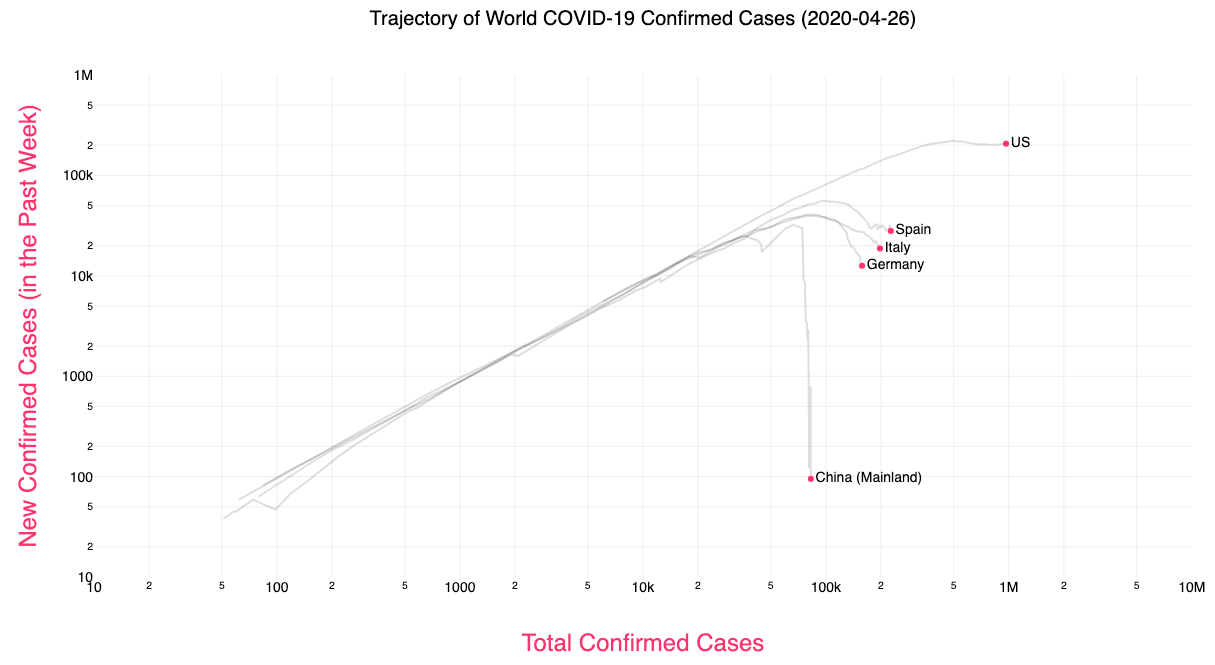
Figure 3: Total confirmed cases vs new cases for US, Spain, Italy, and China (Source: https://aatishb.com/covidtrends/).
Taking a deeper dive into the data, we can look at the cumulative cases over time for Germany and compare it to the plot in Figure 3. Figure 4 below illustrates how the drop in new cases (left plot) is a more discernible sign that the epidemic is slowing than the cumulative progression of the virus (right plot).
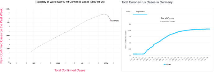
Figure 4: Side-by-side view of two different ways to look at the COVID-19 epidemic in Germany. Source of plot on the right is: https://www.worldometers.info/coronavirus/country/germany/
We are in this together
By selecting all countries on the COVID trends website, COVID-19 progression exhibits very similar dynamics across the globe. This clearly shows this is a pandemic that severely impacts all countries. Countries and regions that are not yet overwhelmed can prepare based on experiences from the hotspot regions
By looking at the progression of the epidemic in different ways, we can start learning more about how the epidemic grows and estimate when the number of cases starts to decrease. It is encouraging when watching, for example, Governor Cuomo of New York analyze the daily increases in deaths and new cases. While this analysis is not exactly the view we use in Figure 3 and on the Covid Trends website, examining daily increases in deaths and cases are useful barometers for the outbreak’s timeline. When those daily increases subside is when the exponential nature of the outbreak begins to plateau. Modeling and visualizing the pandemic will hopefully improve our preparedness for any future waves.
Sources
- California, S. (2020). Stay home except for essential needs. Retrieved 28 April 2020, from https://covid19.ca.gov/stay-home-except-for-essential-needs/
- Cumulative Cases. (2020). Retrieved 28 April 2020, from https://coronavirus.jhu.edu/data/cumulative-cases
- Ma, J. (2020). Estimating epidemic exponential growth rate and basic reproduction number. Infectious Disease Modelling, 5, 129-141. doi: 10.1016/j.idm.2019.12.009
- Paul LeBlanc, C. (2020). Fauci: ‘You don’t make the timeline, the virus makes the timeline’ on relaxing public health measures. Retrieved 28 April 2020, from https://www.cnn.com/2020/03/25/politics/anthony-fauci-coronavirus-timeline-cnntv/index.html
- Covid Trends. (2020). Retrieved 28 April 2020, from https://aatishb.com/covidtrends/
- (2020). Retrieved 28 April 2020, from https://www.youtube.com/watch?v=54XLXg4fYsc
- Germany Coronavirus: 158,758 Cases and 6,126 Deaths – Worldometer. (2020). Retrieved 28 April 2020, from https://www.worldometers.info/coronavirus/country/germany/
- Sheridan, J. (2020). FILE: Slides from Cuomo’s 4/7 coronavirus briefing presentation. Retrieved 29 April 2020, from https://www.news10.com/news/ny-news/file-slides-from-cuomos-4-7-coronavirus-briefing-presentation/
- Caroline Kelly and Jen Christensen, C. (2020). CDC chief says there could be second, possibly worse coronavirus outbreak this winter. Retrieved 29 April 2020, from https://www.cnn.com/2020/04/21/politics/second-coronavirus-cdc-director-robert-redfield/index.html